[Classical Control]Controller Design: Time Response(Transient Response)_2

1. Introduction

이번 포스팅은 Transient response를 Pole과 Zero의 관점에서 살펴볼 것이다. 대표적으로 Dominant pole, Pole-zero cancellation에 대해 다룰 것이다. 특히 필자가 설계하는 PMSM current controller의 Equivalent RL circuit은 Pole-zero cancellation을 반영하여 구현하기 때문에 상당히 중요한 개념이다.

 

2. The Dominant Pole

Dominant pole은 Pole이 3개 이상인 Higher-order system을 Lower-order system와 같은 간단한 시스템으로 근사화하기 위해 활용하는 개념이다. 이때 근사화가 가능한 Pole을 Nondominant pole 혹은 Moveable pole이라고 하고, Controller design의 Performance를 결정하는 Imaginary axis에 가까운 Pole을 Dominant pole 혹은 Fixed pole이라고 한다. 간단하게 Equation 1.과 같은 Third-order system C(s)의 Step response가 Complex poles와 Real pole로 이루어져 있다고 하자.

Equation 1.

이를 Time domain에서 Equation 2.처럼 표현할 수 있다.

Equation 2.

Figure 1. Pole Plot

Figure 1.의 Case 1의 경우 Complex poles이 Real pole과 크게 차이가 안나는 경우이다. 위에서 보는 것처럼, Real pole이 Step response에 미치는 영향이 상당히 크다고 할 수 있다. Case 2는 Real pole의 절댓값 크기가 Complex poles의 Real part의 절댓값 크기보다 훨씬 큰 경우이다. Case 3이 Complex poles만 존재하는 경우라고 볼 수 있는데 Case 2와 크게 차이가 나지 않는다는 것을 알 수 있다. 따라서 Case 2의 Performance의 경우 Case 3처럼 근사화(Approximation)하여 Controller를 설계한다. 통상 Real pole의 절댓값 크기가 Complex poles의 Real part의 절댓값 크기보다 5배 정도 클 때 근사화를 적용한다.

pole = 15
numpole = 100*pole;
denpole = conv([1 pole],...
[1 4 100]);
Ta = tf (numpole,denpole);
num = 100;
den = [1 4 100];
T = tf(num,den);
step(Ta,'.',T,'-')
title('When pole is far away')
legend()

Figure 2. Faraway Pole

Figure 2.는 Real pole과 Complex poles가 멀리 떨어져 있을 때 Dominant pole approximation을 적용했을 때이다. 또한 Figure 3.처럼 멀리 떨어지지 않았을 때의 관계도 확인할 수 있다.

pole = 4
numpole = 100*pole;
denpole = conv([1 pole],...
[1 4 100]);
Ta = tf (numpole,denpole);
num = 100;
den = [1 4 100];
T = tf(num,den);
step(Ta,'.',T,'-')
title('When pole is far away')
legend()

Figure 3. Close Pole

이러한 Dominant pole도 Pole-zero cancellation이 되는 간단한 근사화 형태와 시스템이 Critically damped 될 경우 사용하기 어렵다는 문제점을 안고 있다. 따라서 설계 시에 Controller의 변수에 따라 적절한 기법을 선정해야 하며 Dominant pole 기법만이 정답은 아니다.

 

3. Effect of Zero

시스템에서 Zero는 Residue로 작용하여 Amplitude에 영향을 준다. 이러한 Zero도 크기와 부호에 따라 System에 많은 영향을 주게 되며 우선 Zero의 크기에 따른 영향을 살펴보자.

deng=[1 2 9];
Ta=tf([1 3]*9/3,deng);
Tb=tf([1 5]*9/5,deng);
Tc=tf([1 10]*9/10,deng);
T=tf(9,deng);
step(T,Ta,Tb,Tc)
text(0.5,0.6,'no zero')
text(0.4,0.7,...
'zero at -10')
text(0.35,0.8,...
'zero at -5')
text(0.3,0.9,'zero at -3')
title('Effect of Zero')

Figure 4. Effect of Zero Amplitude

우선 LHP에서 Zero는 절댓값의 크기가 커질수록 Overshoot이 증가한다는 것을 확인할 수 있다. 이와 반대로 Zero가 RHP에 배치될 경우(Positive zero)에는 Figure 5.처럼 Step response에서 Nonminimum-phase 현상이 나타나게 된다.

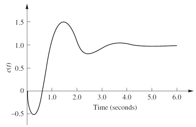
Figure 5. Step Response of a Nonminimum-Phase System

 

4. Pole-Zero Cancellation

Pole-Zero Cancellation은 PMSM의 Current controller를 설계할 때 가장 많이 사용되는 기법이다. Pole-zero cancellation은 수학적으로 Pole과 Zero를 같도록 만들어 약분시키는 개념이다. Open-loop transfer function을 1로 만들어 시스템Input과 Output을 최대한 추종하게 만드는 것이 목적이다. Transfer function T(s)가 있다고 할 때, Real pole P3과 Zero인 z의 Cancellation을 Equation 3.처럼 표현할 수 있다.

Equation 3.

실제 Controller를 설계하면 Zero와 Pole은 현장에서 무조건 오차가 존재할 수밖에 없다. Third-order system을 Second-order system으로 Pole-zero canclellation 해도 실제로는 Second-order system과 비슷한 Third-order system이라는 것이다. 현장에서는 이러한 오차를 Feedback controller를 통해서 어느 정도 감수하고 설계를 진행한다.

Figure 6. PMSM Pole-Zero Cancellation

Figure 6.처럼 PMSM 제어 시에 RL 변수인 Inductance L 값과 Resistance R 값을 파악하고, P controller를 R 값, I controller를 L 값과 같은 비로 두어 Pole-Zero cancellation 한다.

 

* Reference

Figures: Nise, N. S. (2015). Control systems engineering.
Dominant Pole Concept: https://lpsa.swarthmore.edu/PZXferStepBode/DomPole.html
Github Simulation: https://github.com/TitusChoi/Classical_Control/