[Classical Control]Controller Design: Time Response(Transient Response)_1

1. Introduction

이번 포스팅에서는 Controller design시에 Efficient에 가장 큰 영향을 미치는 요소인 Transient response에 대해 알아볼 것이다. 특히 Time domain에서 관찰할 수 있는 Rise time, Settling time, Overshoot, Peak time의 정의와 이에 대한 Poles의 움직임을 살펴보겠다.

 

2. First-Order System

Figure 1.a. First-Order System; b. Bode Plot 

Figure 1.과 같은 First-order system이 있을 때, 이에 대한 Time domain에서 시스템을 분석하는 방법인 Step response를 활용하여 Pole인 a의 특성을 살펴보자. 이때 Step response는 C(s)이다.

Equation 1.

여기 Inverse Laplace transform을 취해보면 Equation 2.와 같은 Step response를 구할 수 있으며, Step input 1을 제외한 나머지 출력이 시스템의 Natural response이다.

Equation 2.

이때 시스템의 Pole인 a의 역수, 즉 1/a을 Time constant(시정수)라고 부르며 다음과 같은 관계식을 도출할 수 있다.

Equation 3.

Equation 3.의 a에 따라 First-order system의 Transient performance가 결정된다.

Figure 2. First-Order System Response to a Unit Step Input

First-order system의 Final value 10%부터 90%에 도달하기까지 걸린 시간을 Rise time Tr이라고 정의하며, Final value의 2% 이내 수렴하기까지 걸리는 시간을 Settling time Ts라고 정의한다.

2.1. Rise Time

Rise time은 Threshold를 정하기 나름이지만, 보통의 경우 Final value의 10%에서 90% 도달할 때까지의 시간을 의미한다. 정의에 따라, c(t)=0.9일 때 t를 c(t)=0.1일 때 t에서 빼주면 되고, 따라서 Equation 4.와 같이 정리된다.

Equation 4.

2.2. Settling Time

마찬가지로 Settling time은 Final value의 2% 내에 도달하는 시간을 구하는 것이기 때문에 c(t)=0.98을 적용해서 구한다.

Equation 5.

MATLAB에는 Transfer function의 Rise time, Settling time을 간편하게 구할 수 있는 'stepinfo' 함수가 있다. 특히 Rise time의 Threshold도 정할 수 있다.

s = tf('s');
H = 50/(s+50)
step(H), grid on
H_info = stepinfo(H)

Figure 3. Step Response Information

2.3. Bandwidth

First-order system에서 Bandwidth는 'the magnitude response curve is 3 dB down from its value at zero frequency'로 정의되며 Equation 6.과 같이 표현할 수 있다. Bandwidth는 Rise time과 마찬가지로 시스템의 응답성을 보는 요소이다. 일반적으로 Bandwidth가 넓을수록 시스템 응답성이 좋아지며, Distortion이 일어나지 않는다. 

Equation 6.

 

3. Second-Order System

Second-order system을 논하기 전에 이전에 간단하게 설명했던 Second-order system의 종류에 대해 알아보자. Underdamped system에서 정의했던 Damping ratio에 따라 Figure 4.처럼 4가지로 나눌 수 있다.

Figure 4. Second-Order System of Damping Ratio

3.1. Undamped System(Damping Ratio=0)

Undamped system은 두 개의 Imaginary poles가 존재하는 형태이고, Equation 7.처럼 형성된다.

Equation 7.

3.2. Underdamped System(Damping Ratio=1)

Underdamped system은 두 개의 Complex poles가 존재하는 형태이고, Equation 8.처럼 형성된다.

Equation 8.

3.3. Critically Damped System(0<Damping Ratio<1)

Critically damped system은 Repeated Poles가 존재하는 형태이고, Equation 9.처럼 형성된다.

Equation 9.

3.4. Overdamped System(Damping Ratio>1)

Overdamped system은 두 개의 Real poles가 존재하는 형태이고, Equation 10.처럼 형성된다.

Equation 10.

 

4. Underdamped Second-Order System

Second-order system 중 Underdamped 조건(Pole이 Stable)에서 시스템 설계를 진행하기 때문에 Underdamped second-order system 특성이 가장 중요한 설계 조건이 된다. Underdamped second-order system이 Equation 11.이라고 할 때 이에 대한 Step response c(s)를 살펴보자.

Equation 11.

이를 Inverse Laplace transform을 활용하여 Time domain에서 관찰하면 Equation 12.처럼 정리할 수 있다.

 

Equation 12.

Underdamped system의 Transient response 향상은 Rise time Tr, Peak time Tp, Overshoot %OS, Settling time Ts의 특성을 본다.

Figure 5. Underdamped System

4.1. Rise Time

First-order system과 마찬가지 정의로 Rise time Tr은 c(t)=0.1부터 c(t)=0.9가 되기까지의 시간을 말하며 Equation 13.과 같이 정의된다.

Equation 13.

4.2. Peak Time

Peak time은 Figure 5.에서 c(t)=cmax에 도달했을 때 시간을 의미하며, Equation 14.와 같이 정의된다.

Equation 14.

4.3. Overshoot(%OS)

Overshoot은 최대 Peak 값과 Final value를 비교하기 위해 사용되는 정의이며, 이 비율이 낮을수록 좋다. Equation 15.와 같이 정의한다.

Equation 15.

이를 정리하면, Equation 16.과 같이 도출된다.

Equation 16.

4.4. Settling Time

Settling time은 Steady-state 상황에서 2% 내에 수렴할 때의 시간을 의미한다. 이 값에 근거하여 Equation 17.처럼 근사적으로 정의된다.

Equation 17.

마찬가지로 'stepinfo'를 활용해서 Second-order system의 특성도 관찰할 수 있다.

s = tf('s');
H = 25/(s^2+5*s+25)
step(H), grid on
H_info = stepinfo(H)

Figure 6. Step Response Information

Figure 7.은 Poles의 움직임에 따른 Step response 변화이다. 이에 근거하여 Closed-loop system의 Controller를 설계한다.

Figure 7. Poles Move

4.5. Bandwidth

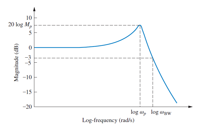
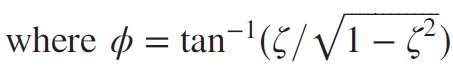
Figure 8. Log-Magnitude Plot

Second-order system에서 Bandwidth는 마찬가지로 'the magnitude response curve is 3 dB down from its value at zero frequency'로 정의되며 Equation 18.과 Figure 8. 같이 표현할 수 있다. Bandwidth는 Rise time과 마찬가지로 시스템의 응답성을 보는 요소이다. 일반적으로 Bandwidth가 넓을수록 시스템 응답성이 좋아지며, Distortion이 일어나지 않는다. 

Equation 18.

 

* Reference

Figures & Theories: Nise, N. S. (2015). Control systems engineering.
MATLAB Function: https://kr.mathworks.com/help/control/ref/lti.stepinfo.html
Github Simulation: https://github.com/TitusChoi/Classical_Control/